
Calculate Friction Loss and Pressure Drop in Any Pipe
Darcy–Weisbach equation + Colebrook friction factor, in SI or US units
Pressure drop is the pressure a fluid loses as it flows through a pipe. Most of it comes from friction against the pipe wall; the rest comes from fittings, valves and any change in height. This calculator uses the Darcy–Weisbach equation with the Colebrook friction factor, the method taught in university fluid mechanics and used in everyday piping design. Enter the fluid, pipe and flow, and it returns velocity, Reynolds number, friction factor, friction loss, fitting losses and the total pressure drop.
Pipe Pressure Drop Calculator
Full, circular pipe · single-phase Newtonian fluid · steady flow · constant diameter
| Flow velocity v | — |
|---|---|
| Flow rate Q | — |
| Reynolds number Re | — |
| Flow regime | — |
| Relative roughness ε/D | — |
| Darcy friction factor f | — |
| Dynamic pressure ρv²/2 | — |
| Friction loss in straight pipe | — |
| Fittings and valves (ΣK = 0) | — |
| Elevation (hydrostatic) | — |
| Total | — |
| Total as head of fluid | — |
Where your flow sits on the Moody diagram
Solid grey curves: turbulent friction factor for fixed ε/D (smooth, 10⁻⁵, 10⁻⁴, 10⁻³, 0.01, 0.05). Blue: laminar line f = 64/Re. Dashed green: your ε/D. Shaded band: transitional flow, 2300 < Re < 4000.
Educational and estimating tool. Results are accurate for the stated assumptions, but real systems add uncertainty: pipe roughness changes with age, fitting K-values vary by manufacturer, and fluid properties change with temperature.
For safety-critical, code-regulated or contractual design, confirm with manufacturer data and the applicable standard (for example ASME B31.3 for process piping).
How to Use the Calculator
- Pick the fluid. Choose water at its temperature, air, or oil, or choose “Custom” and type the density and dynamic viscosity yourself. Viscosity of liquids falls sharply as they warm up, so the temperature matters.
- Enter the pipe. Use the inside diameter, the length, and a material. The material sets the roughness; you can overwrite it if you know the actual value.
- Enter the flow. Give either the flow rate or the mean velocity. If you know the flow rate, the calculator finds the velocity from the pipe area.
- Add elevation and fittings. Enter the height difference between outlet and inlet, then the number of each fitting. Skip these for a straight, level run.
- Read the results. Check the flow regime first: a laminar, transitional or turbulent label tells you which friction-factor method applies. Then read the friction loss, fittings loss, and total.
Tip: Changing a unit drop-down converts the number in that field, so the physical value stays the same. The “SI / US customary” switch changes every unit at once.
Worked Example: Water in a Steel Pipe
Problem. Water at 20 °C flows at 3.0 L/s through 100 m of horizontal commercial-steel pipe with an inside diameter of 50 mm. There are no fittings. Find the pressure drop.
| Quantity | Value | Source |
|---|---|---|
| Density ρ | 998.2 kg/m³ | Water at 20 °C |
| Dynamic viscosity μ | 1.002 mPa·s = 1.002×10⁻³ Pa·s | Water at 20 °C |
| Inside diameter D | 0.050 m | Given |
| Length L | 100 m | Given |
| Flow rate Q | 3.0 L/s = 0.0030 m³/s | Given |
| Roughness ε | 0.045 mm = 4.5×10⁻⁵ m | Commercial steel |
- Pipe area.
A = πD²/4 = π × 0.050² / 4 = 1.9635×10⁻³ m²
- Velocity.
v = Q / A = 0.0030 / 1.9635×10⁻³ = 1.528 m/s
- Reynolds number.
Re = ρvD/μ = 998.2 × 1.528 × 0.050 / 1.002×10⁻³ = 76,105Re is well above 4000, so the flow is turbulent.
- Relative roughness.
ε/D = 0.045 mm / 50 mm = 9.0×10⁻⁴
- Friction factor (Colebrook, solved by iteration).
1/√f = −2 log₁₀[ ε/(3.7D) + 2.51/(Re√f) ] → f = 0.02249Cross-check with the explicit Swamee–Jain formula: f = 0.02264 (+0.7%).
- Dynamic pressure.
ρv²/2 = 998.2 × 1.528² / 2 = 1,165 Pa
- Darcy–Weisbach.
ΔP = f × (L/D) × ρv²/2 = 0.02249 × (100/0.050) × 1,165 = 52,400 Pa
Result: ΔP ≈ 52.4 kPa (0.524 bar, 7.60 psi). As a head of water that is 52,400 / (998.2 × 9.80665) = 5.35 m (17.6 ft).
A pump feeding this pipe must supply at least this pressure, plus any pressure needed at the outlet.
Second check: laminar flow of oil
Hydraulic oil (ISO VG 46 at 40 °C, ρ ≈ 870 kg/m³, μ ≈ 0.040 Pa·s) moves at 1.0 m/s through 20 m of 25 mm smooth tube. Here Re = 870 × 1.0 × 0.025 / 0.040 = 544, so the flow is laminar and f = 64/Re = 0.1177. The result, ΔP = 40.96 kPa, matches the exact Hagen–Poiseuille formula ΔP = 32μLv/D² = 40,960 Pa. Laminar friction does not depend on roughness.
What Is Pressure Drop in a Pipe?
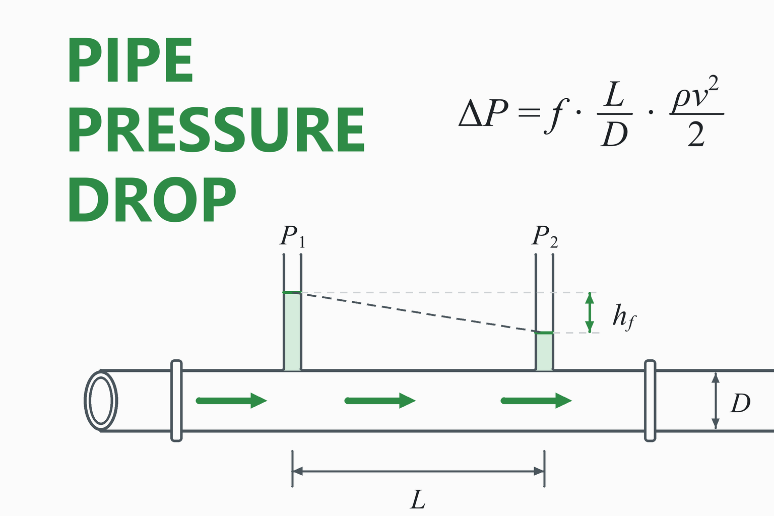
A moving fluid is slowed by friction where it touches the pipe wall. That friction is passed inward through the fluid’s own internal friction (viscosity), so the whole stream feels a drag. Something has to overcome that drag: a pump, gravity, or a pressure difference between the two ends. The pressure that is used up along the way is the pressure drop, also called friction loss. Expressed as a height of fluid instead of a pressure, it is called head loss.
Pressure drop matters because it decides:
- how big a pump you need, and how much electricity it uses;
- whether enough pressure is left at the far end of a system;
- what pipe diameter is a sensible compromise between pipe cost and pumping cost;
- whether velocity is low enough to avoid noise, erosion and pressure surges.
Friction (major) loss
Caused by wall friction along the straight pipe. It grows with length and velocity, and shrinks quickly as diameter increases.
Minor losses
Caused by elbows, tees, valves, entrances and exits, where the flow separates and mixes. “Minor” is a name, not a promise: in short pipes they can dominate.
Elevation change
Pushing fluid uphill costs pressure of ρ·g·Δz, even if no friction acts. Going downhill gives that pressure back.
Pressure and head are the same thing in different units
With ΔP in pascals, ρ in kg/m³, g = 9.80665 m/s² and h in metres. For water, 1 bar ≈ 10.2 m of head and 1 psi ≈ 0.70 m of head.
The Darcy–Weisbach Equation
For a full circular pipe, the friction pressure drop is the dynamic pressure of the flow, multiplied by the length of pipe measured in diameters, multiplied by a dimensionless friction factor:
Darcy–Weisbach (pressure form)
Darcy–Weisbach (head form)
| Symbol | Meaning | SI unit |
|---|---|---|
| ΔPf | Friction pressure drop | Pa |
| f | Darcy friction factor (dimensionless) | – |
| L | Pipe length | m |
| D | Inside diameter | m |
| ρ | Fluid density | kg/m³ |
| v | Mean velocity, v = Q/A = 4Q/(πD²) | m/s |
| g | Gravitational acceleration, 9.80665 | m/s² |
Darcy or Fanning? Some books use the Fanning friction factor, which is one quarter of the Darcy factor. The equation above is for the Darcy factor. Mixing the two gives an answer that is wrong by a factor of four.
What the equation tells you
- Length: double the pipe and you double the friction loss.
- Velocity: in rough or high-Re flow, double the flow and the loss is about four times larger (v²). In smooth pipes at moderate Re the exponent is closer to 1.75, because f also falls as Re rises.
- Diameter: for a fixed flow rate, ΔP varies roughly as 1/D⁵. A pipe 10% larger in diameter has about 38% less friction loss; doubling the diameter cuts it to roughly 1/32. This is why diameter is the strongest lever in pipe sizing.
Reynolds Number and Flow Regime
The Reynolds number compares inertia with viscosity. It tells you whether the flow moves in smooth layers or in chaotic eddies, and that decides how friction behaves.
Reynolds number
ν = μ/ρ is the kinematic viscosity (m²/s). Re is dimensionless, so ρ, v, D and μ must be in consistent units.
| Regime | Reynolds number | What happens | Friction factor |
|---|---|---|---|
| Laminar | Re < 2300 | Smooth, parallel layers. Wall roughness has no effect. | f = 64/Re |
| Transitional | 2300 – 4000 | Flow flips between laminar and turbulent. Unstable and hard to predict. | Uncertain |
| Turbulent | Re > 4000 | Eddies mix the fluid. Friction depends on Re and roughness. | Colebrook |
Water in an ordinary pipe is almost always turbulent: for 50 mm pipe, Re passes 4000 at only about 0.08 m/s. Laminar flow is common for oils, glycols and other viscous liquids, and in very small tubes.
Transitional flow (2300 < Re < 4000). No formula is reliable here. This calculator uses the turbulent (Colebrook) value, which is higher than the laminar value at the same Re and therefore errs on the safe side for pump sizing, and it shows a warning. If your design sits in this band, change the flow or the pipe size if you can.
The Friction Factor: From Laminar Flow to Colebrook
Laminar flow
For laminar flow the friction factor can be derived exactly from the equations of fluid motion (Hagen–Poiseuille flow):
Substituting this into Darcy–Weisbach gives the Hagen–Poiseuille result ΔP = 32 μ L v / D², which depends on viscosity, not on density or roughness.
Turbulent flow
For turbulent flow there is no exact solution, so f is found from experiments. The standard correlation is the Colebrook equation (1939), which is the basis of the Moody diagram (1944):
Colebrook equation
f appears on both sides, so it must be found by iteration. This calculator starts from a guess and repeats the calculation until the value stops changing (to 13 decimal places).
The two terms inside the bracket show the physics. The first, ε/(3.7D), is the effect of wall roughness. The second, 2.51/(Re√f), is the effect of viscosity. At low Re the second term dominates and the pipe behaves as if smooth. At very high Re it vanishes, and f depends only on ε/D (the “fully rough” limit).
Explicit alternative: Swamee–Jain (1976)
Within about 1% of Colebrook for 5,000 ≤ Re ≤ 10⁸ and 10⁻⁶ ≤ ε/D ≤ 10⁻², and easy to use in a spreadsheet without iteration.
The Moody diagram in the calculator above plots your flow on these curves, so you can see how close you are to the laminar or fully rough limits.
Minor Losses: Fittings and Valves
Each fitting disturbs the flow and causes a loss that is proportional to the dynamic pressure. It is written with a loss coefficient K:
An equivalent way to think of it: a fitting adds the friction of a length Le = K · D / f of straight pipe (the “equivalent length”). The calculator shows this total.
| Fitting | K |
|---|---|
| Pipe entrance, sharp-edged | 0.5 |
| Pipe entrance, well-rounded (large radius) | 0.03 |
| Pipe exit into a tank or open space | 1.0 |
| 90° elbow, flanged, regular | 0.3 |
| 90° elbow, threaded, regular | 1.5 |
| 45° elbow, threaded, regular | 0.4 |
| Tee, flow through the run (flanged) | 0.2 |
| Tee, flow through the branch (flanged) | 1.0 |
| Gate valve, fully open | 0.2 |
| Ball valve, fully open | 0.05 |
| Globe valve, fully open | 10 |
| Swing check valve, forward flow | 2 |
The pipe-exit coefficient of 1.0 means that all the kinetic energy of the stream is lost when it discharges into a tank. If the pipe discharges to atmosphere as a free jet, the exit is usually treated differently (as velocity head), so check which one your problem means.
Pipe Roughness Values
| Material | ε (mm) | ε (in) |
|---|---|---|
| Drawn tubing: copper, brass, glass, PVC, plastic | 0.0015 | 0.00006 |
| Commercial steel, wrought iron | 0.045 | 0.0018 |
| Asphalted cast iron | 0.12 | 0.0047 |
| Galvanized iron | 0.15 | 0.0059 |
| Cast iron (new) | 0.26 | 0.0102 |
Fluid Properties Used by the Calculator
| Fluid | Density ρ (kg/m³) | Dynamic viscosity μ (mPa·s) |
|---|---|---|
| Water, 10 °C | 999.7 | 1.307 |
| Water, 20 °C | 998.2 | 1.002 |
| Water, 40 °C | 992.2 | 0.653 |
| Water, 60 °C | 983.2 | 0.467 |
| Water, 80 °C | 971.8 | 0.355 |
| Air, 20 °C, 1 atm | 1.204 | 0.01825 |
| Hydraulic oil ISO VG 46, 40 °C (approximate) | 870 | 40 |
Rule-of-thumb velocities. For water in steel pipe, designers often aim for roughly 1–3 m/s in discharge lines and lower, around 0.5–1.5 m/s, on pump suction lines. These are common guidelines, not limits; the right value depends on the application, noise, erosion and the governing standard.
Common Mistakes
Using nominal pipe size
A “2 inch” Schedule 40 steel pipe has an inside diameter of 2.067 in (52.5 mm). Because ΔP varies as 1/D⁵, a small diameter error becomes a large pressure error.
Mixing units
Entering millimetres where metres are expected is the classic error. Use the unit drop-downs and let the calculator convert.
Mixing friction factors
Fanning f is ¼ of Darcy f. Using one with the other’s equation gives a factor-of-four error.
Ignoring temperature
Water at 80 °C has only about a quarter of the viscosity of water at 10 °C. Viscous liquids such as oils change far more.
Forgetting the fittings
In a short run with several valves and bends, the fittings can cause more loss than the pipe itself.
Using new-pipe roughness for old pipe
Aged, corroded pipe is rougher than new pipe. For existing systems, allow a margin or use measured data.
Assumptions and Limitations
- Incompressible, single-phase fluid. Fine for liquids. For gases it is only reasonable when the pressure drop is small compared with the absolute pressure (a common rule of thumb is under about 10%). Compressed-air lines with larger drops need compressible-flow methods.
- Newtonian fluid. Water, oils, air and most common fluids qualify. Slurries, polymers, paints and similar non-Newtonian fluids do not.
- Steady flow in a full, circular pipe of constant diameter. Reducers, expansions, partially filled pipes (open-channel flow) and pulsating flow are outside the model.
- Fully developed turbulent flow for the Colebrook value, valid for Re up to 10⁸ and ε/D up to 0.05, the range of the Moody diagram. The calculator warns when you leave it.
- Constant fluid properties. Temperature changes along a long pipe change viscosity, and the result changes with it.
- Total pressure drop here is the static pressure difference between inlet and outlet for equal pipe diameters. It does not include pump head, control-valve pressure drop or the pressure needed at the outlet.
How This Calculator Was Verified
The calculation code was tested against results that can be checked independently:
| Check | Expected | Calculator |
|---|---|---|
| Laminar, Re = 1000 | f = 64/Re = 0.0640 | … |
| Smooth pipe, Re = 10⁵ | f ≈ 0.0180 (Colebrook; Moody diagram) | … |
| ε/D = 0.001, Re = 10⁵ | f ≈ 0.0222 (Colebrook; Moody diagram) | … |
| Fully rough, ε/D = 0.01, Re = 10⁸ | f = [2 log₁₀(3.7 D/ε)]⁻² = 0.03790 | … |
| Laminar oil example | ΔP = 32μLv/D² = 40.96 kPa | … |
| Worked example above | Independent SciPy solver: f = 0.022488, ΔP = 52.40 kPa | … |
The “Calculator” column above is computed live by the same code that runs the calculator, in your browser.
Frequently Asked Questions
What is the difference between pressure drop and head loss?
They measure the same energy loss in different units. Pressure drop is in pressure units (Pa, kPa, bar, psi). Head loss is the equivalent height of the flowing fluid (m or ft). They are linked by ΔP = ρ·g·h.
Head is convenient for pumps, because a centrifugal pump’s head does not depend on the fluid density. Pressure is convenient for gauges and for gases.
Which friction factor does this calculator use?
The Darcy friction factor. For laminar flow (Re < 2300) it uses f = 64/Re. For Re of 2300 and above it solves the Colebrook equation by iteration, which accounts for both the Reynolds number and the pipe roughness.
What does the calculator do in transitional flow?
Between Re 2300 and 4000 the flow can switch between laminar and turbulent, and no correlation is reliable. The calculator uses the turbulent (Colebrook) friction factor, which is higher than the laminar value at the same Re, and shows a warning.
Treat the result as an estimate, and avoid designing a system to run in this band if you can.
How does pressure drop change with flow rate?
At high Reynolds number or in rough pipe, f is nearly constant, so ΔP is proportional to velocity squared: doubling the flow gives about four times the pressure drop. In smooth pipe at moderate Re, f falls as Re rises and the exponent is nearer 1.75. In laminar flow, ΔP is directly proportional to the flow.
How does pipe diameter affect pressure drop?
For a fixed flow rate, friction pressure drop varies roughly as 1/D⁵, because velocity falls with D² and the L/D term adds one more factor of D. A pipe 10% larger in diameter has about 38% less friction loss, and a pipe twice as wide has roughly 1/32 of it. This ignores the small change in f.
Can I use this for compressed air or other gases?
Only approximately. The method assumes constant density. For a gas it is acceptable when the pressure drop is small compared with the absolute pressure (a common rule of thumb is under about 10%), using the density at the average pressure. For long compressed-air lines with larger drops, use compressible-flow equations.
Can I use it for rectangular ducts or partly full pipes?
Not directly. For turbulent flow in a full, non-circular duct you can use the hydraulic diameter, Dh = 4A/P, in place of D, and enter the actual mean velocity in velocity mode. This is an approximation and is poor for laminar flow. Partly full pipes and channels need open-channel methods such as Manning’s equation.
Should I use the inside diameter or the nominal pipe size?
Always the inside diameter. Nominal sizes are labels, not dimensions. A 2-inch Schedule 40 steel pipe has an inside diameter of 2.067 in (52.5 mm), and a 2-inch Schedule 80 pipe has about 1.939 in (49.3 mm).
Does the total include the pressure a pump has to supply?
No. The total is the pressure the fluid loses between inlet and outlet. To size a pump, add the pressure needed at the outlet and the losses of other components such as filters, heat exchangers and control valves, then add a margin.
References and Further Reading
- Çengel, Y. A., & Cimbala, J. M. Fluid Mechanics: Fundamentals and Applications. McGraw-Hill. (Pipe flow chapter: friction factor, roughness and minor-loss tables.)
- White, F. M. Fluid Mechanics. McGraw-Hill. (Internal flow, Moody diagram and correlations.)
- Crane Co. Flow of Fluids Through Valves, Fittings, and Pipe, Technical Paper No. 410.
- Colebrook, C. F. (1939). Turbulent flow in pipes, with particular reference to the transition region between the smooth and rough pipe laws. Journal of the Institution of Civil Engineers, 11(4), 133–156.
- Moody, L. F. (1944). Friction factors for pipe flow. Transactions of the ASME, 66(8), 671–684.
- Swamee, P. K., & Jain, A. K. (1976). Explicit equations for pipe-flow problems. Journal of the Hydraulics Division, ASCE, 102(5), 657–664.
Related calculators: Reynolds Number Calculator · Shaft Diameter Calculator · Beam Deflection Calculator · All mechanical engineering calculators